Week 10 - Pandas (Part IV) - Transforming Databases

Liaw Bei Le · May 24, 2021

Pandas - Transforming Databases:

Group by

df.groupby([‘columnname’]).max( )
df2 = df.groupby([‘columnname’]).agg({ })
.join( )
df.groupby([‘columnname’])
- groupings .get_group(‘value’)
- groupings.max( )
- groupings.apply(lambda x: )
- groupings.filter(lambda x: )

Reshaping dataframes

df.pivot(index=’ ‘,columns=’ ‘,values=’ ‘)
df.set_index([‘column1’,’column2’]) then pd.DataFrame(df2.stack( ))
df.unstack( )
df.melt( )
df.pivot_table(index=’ ‘, values=’ ‘)

Merging (merge, join) and concatenating (concat) dataframes

Left Join by using df1.merge(df2,how=’ ‘,on=’ ‘)
Inner Join by using df1.merge(df2,how=’ ‘,left_on=’ ‘,right_on=’ ‘)
Right Join by using df1.merge(df2,how=’ ‘,on=’ ‘)
pd.concat([df1,df2]) and .drop_duplicates( )
df.append( )
df.join( )

Mapping variables into groups

pd.cut( )
.map( )
df[‘columnname’] = pd.Categorical(df[‘columnname’])
pd.get_dummies(df[‘categoricalcolumnname’])

What I learnt:

Transforming Databases

Group by

In a group by, you determine the dimensions you want to group by, then specify an aggregation method.

df.groupby([‘columnname’]).max( ) to group by the selected column and apply the maximum aggregation (result gives us the max for each measurement).
Similar to pivot table in excel by unique values in the column, and returning the corresponding max values for all other columns. Hierarchical column index is created as a result.
```
iris.groupby(['species']).max() 
```
df2 = df.groupby([‘columnname’]).agg({ }) to pass several different types of aggregations to multiple variables. Pass a dictionary with the variables you’re interested in along with their associated aggregations.
```
df = iris.groupby(['species']).agg({'sepal_length':['mean','min','max'],'sepal_width':'count'})
df
```

Example: Create groupby, bar plot
The below all shows the same result of x-axis of cyl & categorised by 2 colours for columns ‘mpg’ and ‘hp’ as bars, with their count on the y-axis

df_cars[['mpg','hp','cyl']].groupby('cyl').sum().plot.bar()

df_cars.loc[:[0,1,2]].groupby('cyl').sum().plot.bar()

df_cars.iloc[:,0:3].groupby('cyl').sum().plot.bar()

df_cars.loc[:,['mpg','hp','cyl']].groupby('cyl').sum().plot.bar()

use .join( ) to concatenate the top and bottom level of our column index to flatten hierarchical indexes for simplicity.
```
df.columns = ['_'.join(col).strip() for col in df.columns.values]
df.reset_index()
df
```
The result combines our variable name with the aggregation used. e.g. the column names change from sepal_length > mean , min , max to sepal_length_mean , sepal_length_min , sepal_length_max

df.groupby([‘columnname’]) specify groupings without first applying any aggregation at all.

groupings .get_group(‘value’) is like a where clause in SQL, filters our data that is a part of the column/ group we specified

  '''Step 1: Create a grouping of dataframe Iris by species''' 
  groupings = iris.groupby(['species'])
  '''Step 2: Now, reference the groupings for aggregating and filtering your data.'''
  '''Let's return the setosa group. This yields all rows in our data with species of setosa.''' 
  groupings.get_group('setosa').head()

we can call aggregate functions like groupings.max( )

  '''gives the maximum values of all the rows in all columns for all the unique items in the group, like a pivot table showing max values'''
  groupings.max()

we can apply Lambda functions to groupings like groupings.apply(lambda x: x.max()). Same output as above.

  '''gives the maximum values of all the rows in all columns for all the unique items in the group, like a pivot table showing max values'''
  groupings.apply(lambda x: x.max())

groupings.filter(lambda x: x[‘columnname’].max() <5) to filter your data frame on an aggregate constraint, similar to a having clause in SQL

  '''filter our data frame for only those species that have a maximum petal length below five'''
  groupings.filter(lambda x: x['petal_length'].max() <5)

Reshaping dataframes

df.pivot(index=’ ‘,columns=’ ‘,values=’ ‘) pivot by identifying the index you want to use, the variable you want to pivot from rows to columns, values you want to populate your data frame. Note, pivot doesn’t perform any kind of aggregation, so the index and columns have to be unique combinations.
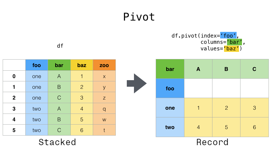
```
'''index shows the unique row indexes, columns shows the unique column names'''
df.pivot(index='Region',columns='Team',values='Revenue')
```

df.set_index([‘column1’,’column2’]) then pd.DataFrame(df2.stack()) to pivot a level of column labels to rows. Work with a multiindex. First we need to set a multi-index for our data frame, by using set index and specifying the columns.

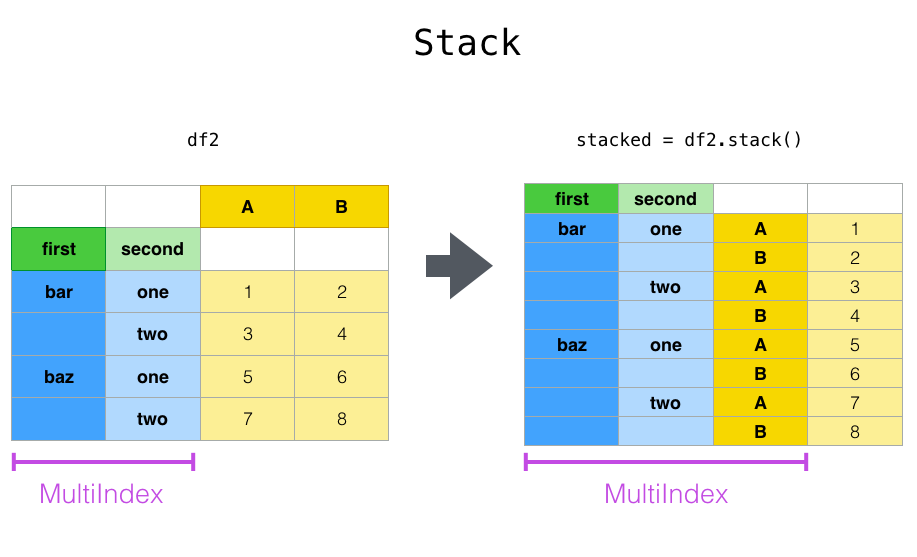
'''set a multi-index for our data frame, use set index and specify region and team'''
df2 = df.set_index(['Region','Team'])
'''call the stack function and create a new data frame called stacked. Now individual rows for the revenue and cost (which were column names previously) and the values for both now lives within the same column.'''
stacked = pd.DataFrame(df2.stack())
stacked

We can reverse the stack process with unstack, that is we’ll pivot level of row labels to columns. The default behavior unstacks all rows, and we can specify at what level in your multi-index you want to unstack.

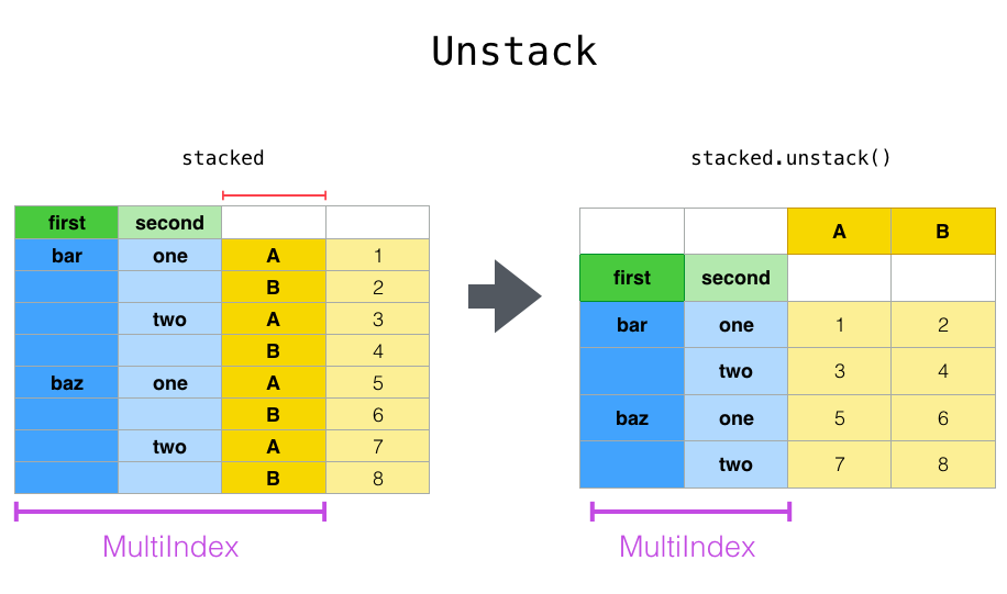
'''all row labels (e.g. revenue and costs) that were stacked previously will unstack to each have their own column once again'''
stacked.unstack()
'''specifically name the index you want to unstack, e.g. region'''
stacked.unstack('Region')

df.melt( ) allows you to reformat your dataframe to identify columns as “ID variables” which will stay intact, while pivoting all other columns, or “measure variables”, from the column to the row level.

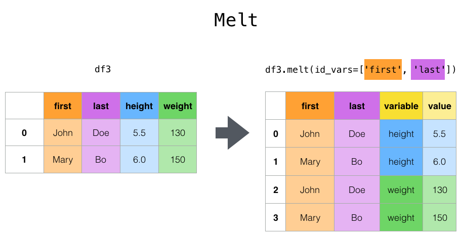
'''designate region and team as our ID variables, then create a new column named "value type" using var_name, and pivot the remaining columns (revenue and cost) back to the row level which will show under 'value type' column we newly created here'''
df.melt(id_vars=['Region','Team'], var_name='value type')

All of the reshaping approaches so far require that we have unique combinations of the row and column variables that we’re pivoting.

If that’s not the case in your data,

df.pivot_table(index=’ ‘, values=’ ‘) e.g. say we had multiple revenue entries for each region and team, you’d want to use pivot table function. Here, we set an index, determine which variables we want pivoted to the columns (if any), then designate our values. By default, pivot table uses mean to aggregate, but you can specify the method you want to use as well.
```
# mean by default
df.pivot_table(index='Team',columns='Region',values='Revenue')
```

Merging (merge, join) and concatenating (concat) dataframes
Merging and combining data from different data frames.

Example dataframes:
Start with 2 different data frames consisting of letters and numbers.
Note the overlap between these two.

df1 = pd.DataFrame({'letter': ['A', 'B', 'C', 'D'],
                    'number': [1, 2, 3, 4]})
df2 = pd.DataFrame({'letter': ['C', 'D', 'E', 'F'],
                    'number': [3, 4, 5, 6]})

Left Join by using df1.merge(df2,how=’ ‘,on=’ ‘)

Specify the join type (in this case a left join) and the join criteria. Here, will match on the ‘number’ column in both data frames.
We see df1 shows up in its entirety and only those letters in df2 that had numbers matching into df1 came through.
```
df1.merge(df2,how='left',on='number')
```
Inner Join by using df1.merge(df2,how=’ ‘,left_on=’ ‘,right_on=’ ‘)

This captures only the overlap between the 2 data frames.
Often the column we’ll be joining on will have different names in our two data sources (not for the example we used here).
In this example, we use left on and right on to specify the join criteria for each of our data frames.
Note: we can join on multiple columns here as well.
```
'''Here, will match on the 'number' column in both data frames.'''
df1.merge(df2,how='inner',left_on='number',right_on='number')
```
Right Join by using df1.merge(df2,how=’ ‘,on=’ ‘)

Opposite of Left Join. We can use the suffixes argument to specify how we want our columns to look after joining. Note that all data from df2, our right data frame was returned along with those that matched from df1.
```
'''Also see the underscore right suffix applied to the letter column from df2.'''
df1.merge(df2,how='right',on='number',suffixes=('','_right'))
```
pd.concat([df1,df2]) to union data frames i.e. essentially stacking them on top of each other (vertically). We can further drop duplicates with .drop_duplicates( )
```
df3 = pd.concat([df1,df2]).drop_duplicates().reset_index(drop=True)
df3
```
To concatenate them horizontally, set axis = 1
```
df4 = pd.concat([df1,df2],axis=1)
df4
```

df.append( ) to append a new row to your dataframe by stacking to data frame vertically. Here we’ll append a series as a new row to our data frame.

'''Append one more row at the bottom with letter Z & number 26.'''
new_row = pd.Series(['Z',26],index=df3.columns)
df3.append(new_row,ignore_index=True)

df.join( ) to join data frames side by side using their index values.
We’ll create another data frame then join that to our df.
We don’t need to specify the join criteria since it will be matching by index but we do need to add in a suffix for repeated column names
(if column names in both df have duplicate names, best to use suffix for the second df we are joining to the first df so the column names won’t clash with the first df).
```
'''create new dataframe'''
join_df = pd.DataFrame({'letter': ['F','G', 'H', 'I'],
                      'number': [6, 7, 8, 9]})
'''join the new df to a df we want to join to'''
df2.join(join_df, rsuffix='_right')
```

Mapping variables into groups
Example dataframe:

df = pd.DataFrame({"Species":['Chinook','Chum','Coho','Steelhead','Bull Trout'], 
"Population":['Skokomish','Lower Skokomish','Skokomish','Skokomish','SF Skokomish'], 
"Count":[1208,2396,3220,6245,8216]})
df

pd.cut( ) allows you to create bins (number ranges) for numerical data, then apply those to your data frame.

'''We're going to create bins of 2000 for our count data.'''
'''imported NumPy to make use of np.inf or infinity, for the top end of our buckets.'''
import numpy as np
# numbers between 0-2000 will show 'Low Return', 2000-4000 show 'Below Avg Return' and so on.
bins = [0, 2000, 4000, 6000, 8000, np.inf]
'''label each of the buckets, from low return to high return.'''
labels = ['Low Return', 'Below Avg Return', 'Avg Return', 'Above Avg Return', 'High Return']
'''create a new column in our data frame called count category.'''
'''pass the count column along with the bins and the labels we've created. This creates our buckets.'''
df['Count Category'] = pd.cut(df['Count'], bins, labels=labels)
df

We can create a dictionary and then use .map( ) which maps values in your data frame into groupings.

'''Here, we'll create a dictionary mapping species to its federal endangered species status.'''
fed_status ={"Chinook":"Threatened", "Chum":"Not Warranted", "Coho":"Not Warranted", "Steelhead":"Threatened"}
'''Next, apply the mappings to our species column using map.'''
'''This creates a new column called "Federal Status" with mapped values of endangered species status''' 
df['Federal Status'] = df['Species'].map(fed_status)
df

Pandas has a specific ‘categorical’ data type. Use df[‘columnname’] = pd.Categorical(df[‘columnname’]) to convert our column into ‘categorical’ data type.

'''ordered equals true will make this variable ordinal meaning high return has a higher order'''
'''pass our labels from above to categories'''
df['Count Category'] = pd.Categorical(df['Count Category'], ordered=True, categories=labels)
df['Count Category']

Output:

Name: Count Category, dtype: category
Categories (5, object): ['Low Return' < 'Below Avg Return' < 'Avg Return' < 'Above Avg Return' < 'High Return']

We can even use this ordering to sort our data.

  '''use sort values by the count category column, and it'll be descending'''
  '''we want data to be sorted from the highest return category to the lowest'''
  df.sort_values(by=['Count Category'],ascending=False)

pd.get_dummies(df[‘categoricalcolumnname’]) to convert a categorical variable into a dummy variable by performing what’s called one hot encoding. It’s especially useful for statistics and machine learning. We create a column for each category and place a 1, if that is true, or 0, if not.
```
pd.get_dummies(df['Count Category'])
```

Additional Resource(s):

More about Pandas group by: 1 | 2

Share: Twitter, Facebook