- Linear Regression
- Cost Function
- Gradient Descent
I am learning about Machine Learning via the Youtube video: Linear Regression Machine Learning tutorial by Siraj Raval.
What I learnt:
Linear Regression for Machine Learning
Linear regression: the process of finding a straight line (as by least squares) that best approximates a set of points on a graph
E.g. using a small dataset of student test scores and the amount of hours they studied.
- Intuitively, there should be a relationship right?
- The more you study, the better your test scores should be.
We’re going to use linear regression to prove this relationship.
Graph of actual hours studied against actual test scores:
- x values: amount of hours studied
- y values: their test scores
Prove their relationship mathematically by drawing a line of best fit.
The way to find the line of best fit is using gradient descent.
- Draw a random line
- Compute the error for that line
- Get an error value that says how well fit is the line to the data
- From there, keep drawing a line iteratively until we get the error value to be minimum
FYI, good to know:
Step 0: Get your dataset and import using code
Step 1: Define our hyperparameters
- learning rate
- inital b
- inital m
- number of iterations
Step 2: Train our model
- Step 2a: Compute error for our line

- Compute the error of our line: the error is the sum of the distances of all actual values from the line of best fit, squared
- square the values as we want it to be positive
- doesn’t matter what the actual value is, it’s more about the magnitude of the value and we want to minimise the value over time
- Step 2b: Run gradient descent
- we want to get to the local minima where error is least
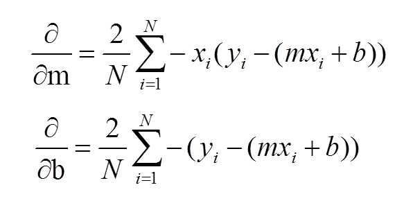
- we need to compute partial derivatives of our error function w.r.t. b and m

#The optimal values of m and b can be actually calculated with way less effort than doing a linear regression.
#this is just to demonstrate gradient descent

from numpy import * # Step 0 import np

# Step 2a Compute error for our line
def compute_error_for_line_given_points(b, m, points):
    totalError = 0 # we don't have an error yet

    # for every training example in our training set
    for i in range(0, len(points)):
        # get the x value
        x = points[i, 0]
        # get the y value
        y = points[i, 1]
        # get the difference, square it, add to total
        totalError += (y - (m * x + b)) ** 2
    # get the average
    return totalError / float(len(points))

# Step 2b(i) run gradient descent
def gradient_descent_runner(points, starting_b, starting_m, learning_rate, num_iterations):
    b = starting_b
    m = starting_m
    for i in range(num_iterations):
        #update b and m with more accurate b and m by performing this gradient step
        b, m = step_gradient(b, m, array(points), learning_rate)
    return [b, m]

# Step 2b(ii) gradient descent step
def step_gradient(b_current, m_current, points, learningRate):

    #starting points for our gradient descent
    b_gradient = 0
    m_gradient = 0
    N = float(len(points))

    # for every single point in our scatter plot of data
    for i in range(0, len(points)):
        x = points[i, 0]
        y = points[i, 1]

        # direction w.r.t. b and m
        # compute partial derivatives of our error function
        b_gradient += -(2/N) * (y - ((m_current * x) + b_current))
        m_gradient += -(2/N) * x * (y - ((m_current * x) + b_current))

    #update our b and m values using our partial derivatives
    new_b = b_current - (learningRate * b_gradient)
    new_m = m_current - (learningRate * m_gradient)
    return [new_b, new_m]

def run():
    # Step 0 Import dataset
    points = genfromtxt("data.csv", delimiter=",")

    # Step 1 Define our hyperparameters
    learning_rate = 0.0001
    # rate of convergence: how fast we can get the line of best fit
    # if too small, slow convergence
    # if too big, error function may not be minimised, may not converge to minima

    initial_b = 0 # initial y-intercept guess
    initial_m = 0 # initial slope guess
    # For all lines, y = mx + b
    # (initial b & m can be any value as we just get a random line first, then work from there.)

    num_iterations = 1000

    # Step 2 Train our model
    # What are the {0},{1},{2}...? We can use index numbers (a number inside the curly brackets { }) to be sure the values are placed in the correct placeholders. https://www.w3schools.com/python/python_string_formatting.asp
    # Show starting b, m and error
    print "Starting gradient descent at b = {0}, m = {1}, error = {2}".format(initial_b, initial_m, compute_error_for_line_given_points(initial_b, initial_m, points))
    print "Running..."

    # Get our optimal line of best fit - print out our final values
    [b, m] = gradient_descent_runner(points, initial_b, initial_m, learning_rate, num_iterations)
    print "After {0} iterations b = {1}, m = {2}, error = {3}".format(num_iterations, b, m, compute_error_for_line_given_points(b, m, points))

run()
